Machine Learning Methods

In this section, we’ll cover the core machine learning methods, including regression, classification, dimensionality reduction, and gradient boosting algorithms. For each method, I’ll provide a practical project idea along with a brief outline of how to solve it using these techniques.

---

1. Regression Algorithms

Overview:

• Regression is used to predict a continuous value based on one or more input features.

• Common Algorithms: Linear Regression, Ridge Regression, Lasso Regression, Polynomial Regression.

Project 1: House Price Prediction

Goal: Predict the price of a house based on features such as the size of the house, number of bedrooms, location, and age.

Dataset: Use the Kaggle House Prices dataset (or any open dataset on house prices).

Solution:

1. Data Preprocessing:

   • Handle missing values.

   • One-hot encode categorical variables (e.g., neighborhood, house style).

   • Normalize numerical features like square footage and lot size.

2. Feature Engineering:

   • Create derived features, such as price per square foot or age of the house.

3. Modeling:

   • Start with Linear Regression and observe performance.

   • Experiment with Ridge Regression and Lasso Regression for regularization to prevent overfitting.

   • If the data is non-linear, try Polynomial Regression.

4. Evaluation:

   • Use Mean Squared Error (MSE) and R-squared as performance metrics.

   • Use cross-validation to check the model’s robustness.

Sample Code:

from sklearn.model_selection import train_test_split
from sklearn.linear_model import LinearRegression, Ridge, Lasso
from sklearn.metrics import mean_squared_error

# Load dataset and preprocess it
# Assume df is a pandas dataframe with processed features and target

X = df.drop('price', axis=1)  # Features
y = df['price']  # Target variable

X_train, X_test, y_train, y_test = train_test_split(X, y, test_size=0.2, random_state=42)

# Train a linear regression model
model = LinearRegression()
model.fit(X_train, y_train)

# Predict and evaluate
y_pred = model.predict(X_test)
mse = mean_squared_error(y_test, y_pred)
print("MSE: ", mse)

---

2. Classification Algorithms

Overview:

• Classification is used to predict a categorical label based on input features.

• Common Algorithms: Logistic Regression, K-Nearest Neighbors (KNN), Support Vector Machines (SVM), Decision Trees, Random Forest.

Project 2: Customer Churn Prediction

Goal: Predict whether a customer will churn (leave) a subscription-based service based on usage patterns, customer support interactions, and demographic data.

Dataset: Use the Kaggle Telecom Customer Churn dataset.

Solution:

1. Data Preprocessing:

   • One-hot encode categorical variables like contract type, payment method, etc.

   • Scale continuous variables like tenure, monthly charges, and total charges.

2. Modeling:

   • Start with Logistic Regression as a baseline.

   • Try Random Forest for a more robust, non-linear approach.

   • Use SVM for high-dimensional feature spaces and KNN for instance-based learning.

3. Feature Engineering:

   • Derive features such as average monthly charges per year of tenure.

4. Evaluation:

   • Use metrics like accuracy, precision, recall, and F1-score.

   • Use ROC-AUC for assessing classification performance.

Sample Code:

from sklearn.model_selection import train_test_split
from sklearn.ensemble import RandomForestClassifier
from sklearn.metrics import accuracy_score, roc_auc_score

# Load dataset and preprocess it
# Assume df is a pandas dataframe with processed features and target

X = df.drop('churn', axis=1)  # Features
y = df['churn']  # Target (binary)

X_train, X_test, y_train, y_test = train_test_split(X, y, test_size=0.2, random_state=42)

# Train a Random Forest model
model = RandomForestClassifier()
model.fit(X_train, y_train)

# Predict and evaluate
y_pred = model.predict(X_test)
accuracy = accuracy_score(y_test, y_pred)
roc_auc = roc_auc_score(y_test, y_pred)
print("Accuracy: ", accuracy)
print("ROC-AUC: ", roc_auc)

---

3. Dimensionality Reduction Algorithms

Overview:

• Dimensionality Reduction is used to reduce the number of features while retaining important information.

• Common Algorithms: Principal Component Analysis (PCA), t-SNE, Linear Discriminant Analysis (LDA), Autoencoders (Neural Networks).

Project 3: Visualizing High-Dimensional Data (MNIST Handwritten Digits)

Goal: Use dimensionality reduction techniques to reduce the dimensionality of the MNIST dataset and visualize the data in 2D.

Dataset: MNIST dataset (available via scikit-learn or Keras).

Solution:

1. Load the MNIST Dataset.

2. Apply PCA to reduce the number of dimensions (e.g., from 784 to 50).

3. Use t-SNE to visualize the data in 2D space, capturing local similarities between the digits.

4. Plot the results using a scatter plot.

Sample Code:

from sklearn.decomposition import PCA
from sklearn.manifold import TSNE
import matplotlib.pyplot as plt
from sklearn.datasets import load_digits

# Load dataset (MNIST)
digits = load_digits()
X = digits.data  # Features (64-dimensional images)
y = digits.target  # Labels

# Apply PCA
pca = PCA(n_components=50)
X_pca = pca.fit_transform(X)

# Apply t-SNE to reduce dimensions to 2D for visualization
tsne = TSNE(n_components=2)
X_tsne = tsne.fit_transform(X_pca)

# Visualize the 2D projection
plt.scatter(X_tsne[:, 0], X_tsne[:, 1], c=y, cmap='tab10')
plt.colorbar()
plt.title('t-SNE Visualization of MNIST Digits')
plt.show()

---

4. Gradient Boosting Algorithms

Overview:

• Gradient Boosting is an ensemble learning technique that combines the predictions of several weak learners to produce a more accurate model.

• Common Algorithms: XGBoost, LightGBM, CatBoost.

Project 4: Predicting Loan Default using XGBoost

Goal: Predict whether a customer will default on a loan based on credit score, income, loan amount, and other financial data.

Dataset: Use any financial dataset with customer loan data (e.g., Kaggle’s Home Credit Default Risk dataset).

Solution:

1. Data Preprocessing:

   • Handle missing values and encode categorical features using one-hot encoding or target encoding.

   • Scale numeric features.

2. Modeling:

   • Use XGBoost for predicting loan defaults. XGBoost is known for its efficiency and performance on tabular data.

3. Feature Importance:

   • After training, use XGBoost’s feature importance to identify the most important features influencing the model’s predictions.

4. Evaluation:

   • Use cross-validation to ensure the model generalizes well.

   • Evaluate performance using accuracy, precision, recall, and ROC-AUC.

Sample Code:

import xgboost as xgb
from sklearn.model_selection import train_test_split
from sklearn.metrics import accuracy_score, roc_auc_score

# Load dataset and preprocess it
# Assume df is a pandas dataframe with processed features and target
X = df.drop('default', axis=1)  # Features
y = df['default']  # Target variable

X_train, X_test, y_train, y_test = train_test_split(X, y, test_size=0.2, random_state=42)

# Train an XGBoost model
model = xgb.XGBClassifier(use_label_encoder=False)
model.fit(X_train, y_train)

# Predict and evaluate
y_pred = model.predict(X_test)
accuracy = accuracy_score(y_test, y_pred)
roc_auc = roc_auc_score(y_test, y_pred)
print("Accuracy: ", accuracy)
print("ROC-AUC: ", roc_auc)

---

Practical problem

Let’s walk through a practical example of using machine learning to build a predictive model. We’ll follow a structured approach that covers the entire machine learning pipeline, including:

1. Problem Definition

2. Data Exploration (EDA)

3. Data Cleaning

4. Feature Engineering

5. Model Selection

6. Model Evaluation

7. Model Tuning

8. Deployment and Monitoring

We’ll use a fictitious problem to keep things straightforward and generalizable. Suppose we are working on predicting whether a customer will churn (i.e., stop using the service) based on customer data for a telecom company.

---

Problem Definition

Objective: Predict whether a customer will churn (yes/no) based on customer data such as demographics, usage patterns, and service history.

Data: You are provided with a dataset containing customer features:

• CustomerID: Unique identifier for each customer.

• Tenure: How long the customer has been with the company.

• MonthlyCharges: The amount billed to the customer monthly.

• TotalCharges: The total amount billed.

• Contract: The type of contract (e.g., month-to-month, one year).

• PaymentMethod: How the customer pays (e.g., credit card, bank transfer).

• Churn: The target variable (1 for churn, 0 for no churn).

---

Step 1: Data Exploration (EDA)

We begin by loading and exploring the data.

import pandas as pd
import matplotlib.pyplot as plt
import seaborn as sns

# Load dataset
data = pd.read_csv('https://github.com/YBIFoundation/Dataset/raw/main/TelecomCustomerChurn.csv')
data = data[['customerID', 'Tenure', 'MonthlyCharges', 'TotalCharges', 'Contract', 'PaymentMethod', 'Churn']]

# Display first few rows
print(data.head())

   customerID  Tenure  MonthlyCharges TotalCharges  Contract  \
0  7590-VHVEG       1           29.85        29.85   Monthly   
1  5575-GNVDE      34           56.95       1889.5  One year   
2  3668-QPYBK       2           53.85       108.15   Monthly   
3  7795-CFOCW      45           42.30      1840.75  One year   
4  9237-HQITU       2           70.70       151.65   Monthly   

               PaymentMethod Churn  
0                     Manual    No  
1                     Manual    No  
2                     Manual   Yes  
3  Bank transfer (automatic)    No  
4                     Manual   Yes  

Initial Checks:

• Summary statistics of numerical features: mean, median, and distribution of each variable.

# Summary statistics
print(data.describe())

# Check for missing values
print(data.isna().sum())

            Tenure  MonthlyCharges
count  7043.000000     7043.000000
mean     32.371149       64.761692
std      24.559481       30.090047
min       0.000000       18.250000
25%       9.000000       35.500000
50%      29.000000       70.350000
75%      55.000000       89.850000
max      72.000000      118.750000
customerID        0
Tenure            0
MonthlyCharges    0
TotalCharges      0
Contract          0
PaymentMethod     0
Churn             0
dtype: int64

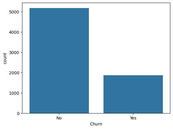
• Class imbalance: Check the distribution of the target variable (Churn). Imbalanced classes could affect model performance.

# Check class distribution
print(data['Churn'].value_counts())
sns.countplot(x='Churn', data=data)
plt.show()

Churn
No     5174
Yes    1869
Name: count, dtype: int64

Visualizing Correlations: Visualize the correlation between numerical features (e.g., tenure, monthly charges) and churn to detect potential patterns.

# Correlation matrix
data['churn'] = data.Churn.map(dict(Yes=1, No=0))
corr = data[['Tenure', 'MonthlyCharges', 'churn']].corr()
sns.heatmap(corr, annot=True, cmap='coolwarm')
plt.show()

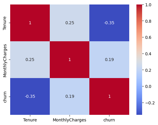
Insights from EDA:

• If the target variable Churn is imbalanced (e.g., 80% no churn, 20% churn), we might need to address this during model training.

• Monthly charges and tenure could show strong correlation with churn, providing clues for feature importance.

---

Step 2: Data Cleaning

We now handle missing data, incorrect formats, and other issues.

# Handle missing values in 'TotalCharges'
# 'TotalCharges' might have some empty strings that need to be converted to NaN and filled.
data['TotalCharges'] = pd.to_numeric(data['TotalCharges'], errors='coerce')

# Fill missing values in 'TotalCharges' with the median
data['TotalCharges'] = data['TotalCharges'].fillna(data['TotalCharges'].median())

Categorical Variable Encoding: For categorical features like Contract and PaymentMethod, convert them to numerical format using one-hot encoding or label encoding.

# One-hot encode categorical variables
data = pd.get_dummies(data, columns=['Contract', 'PaymentMethod'], drop_first=True)

---

Step 3: Feature Engineering

Next, we generate new features and modify existing ones to improve the model’s ability to predict churn.

1. Customer Tenure Grouping: Customers with longer tenures might behave differently, so we can bucket the Tenure feature into categories.

# Create tenure groups
bins = [0, 12, 24, 36, 48, 60, 72]
labels = ['0-12', '12-24', '24-36', '36-48', '48-60', '60-72']
data['TenureGroup'] = pd.cut(data['Tenure'], bins=bins, labels=labels)

2. Interaction Features: Interaction between features like MonthlyCharges and Contract type might provide insight into churn behavior.

# Interaction term between MonthlyCharges and Contract type
data['Charges_Contract'] = data['MonthlyCharges'] * data['Contract_One year']

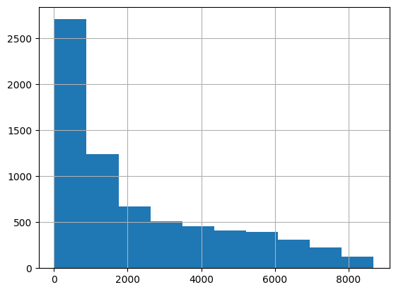
3. Log Transformation: If TotalCharges is highly skewed, applying a log transformation can make the distribution more normal and improve model performance.

data['TotalCharges'].hist()
plt.show()

import numpy as np
data['Log_TotalCharges'] = np.log1p(data['TotalCharges'])

---

Step 4: Model Selection

We now split the data into training and test sets and select candidate models to compare.

from sklearn.model_selection import train_test_split

# Split data into training and test sets
X = data.drop(['Churn', 'churn', 'customerID', 'TenureGroup', 'TotalCharges'], axis=1)  # Features
y = data['churn']  # Target variable

X_train, X_test, y_train, y_test = train_test_split(X, y, test_size=0.2, random_state=42)

Model Choices: We’ll test multiple models, including:

• Logistic Regression (baseline)

• Random Forest

• Gradient Boosting (XGBoost or LightGBM)

from sklearn.linear_model import LogisticRegression
from sklearn.ensemble import RandomForestClassifier
from xgboost import XGBClassifier

# Initialize models
log_reg = LogisticRegression()
rf = RandomForestClassifier()
xgb = XGBClassifier()

# Fit models
log_reg.fit(X_train, y_train)
rf.fit(X_train, y_train)
xgb.fit(X_train, y_train)

/home/qhu/miniconda3/envs/MLbook/lib/python3.12/site-packages/sklearn/linear_model/_logistic.py:469: ConvergenceWarning: lbfgs failed to converge (status=1):
STOP: TOTAL NO. of ITERATIONS REACHED LIMIT.

Increase the number of iterations (max_iter) or scale the data as shown in:
    https://scikit-learn.org/stable/modules/preprocessing.html
Please also refer to the documentation for alternative solver options:
    https://scikit-learn.org/stable/modules/linear_model.html#logistic-regression
  n_iter_i = _check_optimize_result(

XGBClassifier(base_score=None, booster=None, callbacks=None,
              colsample_bylevel=None, colsample_bynode=None,
              colsample_bytree=None, device=None, early_stopping_rounds=None,
              enable_categorical=False, eval_metric=None, feature_types=None,
              gamma=None, grow_policy=None, importance_type=None,
              interaction_constraints=None, learning_rate=None, max_bin=None,
              max_cat_threshold=None, max_cat_to_onehot=None,
              max_delta_step=None, max_depth=None, max_leaves=None,
              min_child_weight=None, missing=nan, monotone_constraints=None,
              multi_strategy=None, n_estimators=None, n_jobs=None,
              num_parallel_tree=None, random_state=None, ...)

In a Jupyter environment, please rerun this cell to show the HTML representation or trust the notebook.
On GitHub, the HTML representation is unable to render, please try loading this page with nbviewer.org.

---

Step 5: Model Evaluation

Evaluate the performance of each model using relevant metrics.

from sklearn.metrics import accuracy_score, classification_report, roc_auc_score

# Make predictions
log_reg_pred = log_reg.predict(X_test)
rf_pred = rf.predict(X_test)
xgb_pred = xgb.predict(X_test)

# Accuracy
print(f"Logistic Regression Accuracy: {accuracy_score(y_test, log_reg_pred)}")
print(f"Random Forest Accuracy: {accuracy_score(y_test, rf_pred)}")
print(f"XGBoost Accuracy: {accuracy_score(y_test, xgb_pred)}")

# Classification Report
print(classification_report(y_test, xgb_pred))

# ROC-AUC Score
print(f"XGBoost ROC-AUC: {roc_auc_score(y_test, xgb_pred)}")

Logistic Regression Accuracy: 0.8005677785663591
Random Forest Accuracy: 0.7693399574166075
XGBoost Accuracy: 0.7970191625266146
              precision    recall  f1-score   support

           0       0.84      0.89      0.87      1036
           1       0.64      0.53      0.58       373

    accuracy                           0.80      1409
   macro avg       0.74      0.71      0.72      1409
weighted avg       0.79      0.80      0.79      1409

XGBoost ROC-AUC: 0.7109862639353256

For imbalanced datasets, focus on metrics like precision, recall, F1 score, and ROC-AUC rather than accuracy alone.

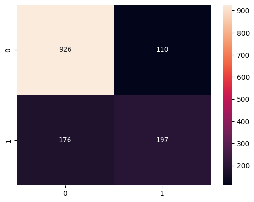
Confusion Matrix:

from sklearn.metrics import confusion_matrix
import seaborn as sns

# Confusion matrix for XGBoost
cm = confusion_matrix(y_test, xgb_pred)
sns.heatmap(cm, annot=True, fmt='d')
plt.show()

---

Step 6: Model Tuning

Once we have a good model, we perform hyperparameter tuning using techniques like Grid Search or Random Search.

from sklearn.model_selection import GridSearchCV

# Hyperparameter grid for XGBoost
param_grid = {
    'n_estimators': [100, 200],
    'max_depth': [3, 4, 5],
    'learning_rate': [0.01, 0.1]
}

# Perform grid search
grid_search = GridSearchCV(estimator=xgb, param_grid=param_grid, cv=5, scoring='roc_auc', verbose=1)
grid_search.fit(X_train, y_train)

# Best parameters
print(grid_search.best_params_)

Fitting 5 folds for each of 12 candidates, totalling 60 fits

{'learning_rate': 0.01, 'max_depth': 5, 'n_estimators': 200}

---

Step 7: Handling Imbalanced Data

Since churn is likely an imbalanced problem, we can address this by:

1. Oversampling the minority class (using SMOTE):

from imblearn.over_sampling import SMOTE

sm = SMOTE(random_state=42)
X_train_smote, y_train_smote = sm.fit_resample(X_train, y_train)

xgb = XGBClassifier()
xgb.fit(X_train_smote, y_train_smote)
xgb_pred_s = xgb.predict(X_test)
print(f"XGBoost ROC-AUC: {roc_auc_score(y_test, xgb_pred_s)}")

XGBoost ROC-AUC: 0.7482454687548522

2. Class weighting (in RandomForestClassifier or XGBoost):

rf = RandomForestClassifier(class_weight='balanced')
xgb = XGBClassifier(scale_pos_weight=(sum(y_train == 0) / sum(y_train == 1)))  # For imbalanced datasets

xgb.fit(X_train, y_train)
xgb_pred_w = xgb.predict(X_test)
print(f"XGBoost ROC-AUC: {roc_auc_score(y_test, xgb_pred_w)}")

XGBoost ROC-AUC: 0.7476541554959786

---

Step 8: Model Deployment and Monitoring

Once the model is trained and tested, we package it for deployment. Using a framework like Flask or FastAPI, we can serve the model predictions through an API.

from flask import Flask, request, jsonify
import pickle

# Load the trained model
with open('xgb_model.pkl', 'rb') as file:
    model = pickle.load(file)

# Initialize Flask app
app = Flask(__name__)

@app.route('/predict', methods=['POST'])
def predict():
    data = request.get_json(force=True)
    prediction = model.predict([data['features']])
    return jsonify({'prediction': int(prediction[0])})

if __name__ == '__main__':
    app.run()

Finally, we monitor the model in production using key performance indicators (KPIs) such as accuracy drift or changes in the distribution of incoming data, ensuring the model continues to perform well.

---

Conclusion

This pipeline outlines a complete approach for building a machine learning model, from data exploration to deployment. It demonstrates a real-world application that includes model tuning, handling imbalanced data, and ensuring deployment-ready code. This structure is typical of how a machine learning engineer would approach building a model end-to-end in a professional setting.